Search This Blog

Showing posts with label Robotics. Show all posts

Wednesday, May 18, 2016

DS1307 Real-time Clock

DS1307 Real-time clock လေးကို အသုံးပြုပုံ အကြောင်း ပြောချင်ပါတယ်။ AliExpress က module လေးဝယ်တာ ၁ ဒေါ်လာလောက်ပဲ ပေးရပါတယ်။ AT24C32 ဆိုတဲ့ 32k EEPROM လေးပါ အဆစ် ပါသေးတယ်။


Figure. Setup.


Thursday, March 24, 2016

Gyroscope L3G4200D

L3G4200D ဆိုတဲ့ STMicroelectronics ကထုတ်တဲ့ MEMS ultra-stable three-axis digital output gyroscope ကို သုံးကြည့်ဖြစ်ပါတယ်။ Aliexpress မှာ ရောင်းတဲ့ L3G4200D Module လေးက ၃ ဒေါ်လာ လောက်ပဲ ပေးရပါတယ်။


Figure. L3G4200 Gyroscope module


Thursday, November 26, 2015

DAC - Digital to Analog Converter

PWM (Pulse Width Modulation) တွေကို analog output တွေအနေနဲ့ အသုံးများပေမယ့် သူတို့က high frequency, high accuracy, hard real-time တွေအတွက်တော့ မသင့်တော်ဘူးလို့ ထင်ပါတယ်။ Analog signal အစစ်မထွက်တဲ့ အတွက် RC low pass filter ခံ သုံးပြန်ရင်လည်း ရလာမယ့် phase lag က hard real-time system တွေမှာ ပြဿနာ အကြီးကြီးပါ။ စျေးပေါ၊ သေးငယ်တဲ့ AD5641 လို DAC လေးတွေက သုံးရလွယ်ကူပြီး အဆင်ပြေတဲ့ solution ပါ။ AD5641 က 3 mm x 2 mm အရွယ်လေးပဲရှိပြီး၊ SPI interface ပါတဲ့ 14 bit DAC ပါ။ Power supply voltage က 2.7 V ကနေ 5.5 V အထိသုံးနိုင်ပါတယ်။ နမူနာ ဆက်သွယ် မှုတခုကို အောက်မှာ ပြထားပါတယ်။

ဒါကတော့ AD5641 တွေကို သုံးထားတဲ့ channel ၃ ခုပါတဲ့ digital to analog converter လေးပါ။ LPC54102 dual core ARM microcontroller ကိုသုံးပြီး AD5641 သုံးခုကို ပြိုင်တူ control လုပ်တဲ့ နမူနာ code ပါ။

Wednesday, November 25, 2015

CC2531 Zigbee USB Dongle

CC2531 USB Evaluation Module Kit ကိုသုံးပြီး wireless communication လုပ်ကြည့်တဲ့ အကြောင်းလေးပါ။ သူ့ရဲ့ website ကိုသွားပြီး CC USB Firmware Library and Examples ဆိုတဲ့ zip ဖိုင်ကို download လုပ်လိုက်ပါတယ်။ ဖိုင်ကိုဖြည်ပြီးတဲ့ အခါ Doc folder ထဲက CC USB Software Examples User’s Guide ထဲမှာ နမူနာပြထားတဲ့ USB RF Modem Example ကို စမ်းကြည့်ခဲ့ပါတယ်။

CC2531 Zigbee Wireless USB Dongle

Tuesday, November 24, 2015

Wireless Communication using CC2530 Zigbee Wireless MCU

CC2530 က IEEE 802.15.4 နဲ့ Zigbee တွေအတွက် RF transceiver နဲ့ 8051 MCU ကို ပေါင်းစပ်ထားတဲ့ system-on-chip (SoC) solution တခုပါ။ သူ့ကို သုံးပြီး wireless module စမ်းလုပ်ဖို့ အတွက် CC2530EM Evaluation Modules နှစ်ခု၊ SmartRF05EB Evaluation Boards နှစ်ခု၊ နဲ့ CC2531 USB Dongle တခုပါတဲ့ CC2530DK devolopment kit ကို ဝယ်တာ USD 400 လောက်ပေးရပါတယ်။ သူတို့နဲ့ သုံးဖို့အတွက် TI ရဲ့ ဝက်ဘ်ဆိုက်မှာ အလကားပေးတဲ့ SmartRF Studio ကို စက်ထဲမှာ install လုပ်ပါတယ်။

CC2530DK

Tuesday, November 17, 2015

Driving 28BYJ-48-5V Stepper Motor with ULN2003A Transistor Arrays on Arduino

28BYJ-48-5V Stepper Motor နဲ့ ULN2003A driver တွေက တော်တော် အသုံးများပုံရပြီး အလွယ်တကူ ဝယ်နိုင်ရုံတင်မက စျေးလည်း တော်တော်ပေါ ပါတယ်။ Stepper Library ကို မသုံးပဲ Arduino ရဲ့ Port B ကို သုံးပြီး Stepper motor ကို ထိန်းတဲ့ ရိုးရှင်းတဲ့ နမူနာလေး ဖော်ပြချင်ပါတယ်။


Figure. Driving 28BYJ-48-5V Stepper Motor with Arduino UNO using USB power.


28BYJ-48-5V Stepper Motor က 5V နဲ့ တိုက်ရိုက်မောင်းနိုင်ပြီး၊ unipolar stepper motor အမျိုးအစားပါ။ သူ့ရဲ့ schematic ကို အောက်မှာပြထားပါတယ်။


Figure. 28BYJ-48-5V Stepper Motor.


ULN2003A Transistor Arrays ကတော့ inductive load တွေကို drive လုပ်ဖို့ ဒီဇိုင်းလုပ်ထားတာမို့ အထဲမှာ free wheeling diode ပါ ပါ ပါတယ်။ Darlington pair သုံးထားတာမို့ အဝင် ဗို့ 1.4V လောက်ကနေ 30V အထိ ကြိုက်တဲ့ ဗို့နဲ့ တိုက်ရိုက်ဆက်ပြီး ထိန်းနိုင်ပါတယ်။


Figure. ULN2003A.


Wave drive, Full step drive နဲ့ Half step drive တွေကို သုံးပြထားတဲ့ နမူနာ ပရိုဂရမ် လေးကို အောက်မှာ ပြထားပါတယ်။


//Driving 28BYJ-48-5V Stepper Motor using ULN2003A Transistor Arrays
//Author: Yan Naing Aye
//Website: http://www.cool-emerald.com/

#include "StepperPortB.h"
//----------------------------------------------------------
void setup() {    
  StepperInit();//setup pins
  //StepperMode(WAVE);
  //StepperMode(FULL);
  StepperMode(HALF);
  //Serial.begin(9600);
}
void loop() {
  Step(4096,2500); //turn 4096 steps forward with 2500 us period for each step
  Step(-4096,2500);//turn 4096 steps backward with 2500 us period for each step
  //Serial.println(CS);
}


//File: StepperPortB.h
//Author: Yan Naing Aye
//Website: http://www.cool-emerald.com/

//Driving 28BYJ-48 – 5V Stepper Motor using ULN2003A Transistor Arrays
//----------------------------------------------------------
#ifndef StepperPortB_h
  #define StepperPortB_h
  #include "Arduino.h"
byte* S; //Stepping sequence

//Wave drive
//Step          0 | 1 | 2 | 3 | 0 |...

//Blue   = A :  1 | 0 | 0 | 0 | 1 | ...
//Pink   = B :  0 | 1 | 0 | 0 | 0 | ...
//Yellow = C :  0 | 0 | 1 | 0 | 0 | ...
//Orange = D :  0 | 0 | 0 | 1 | 0 | ...
byte Wave[4] = {0x01,0x02,0x04,0x08};

//Full Step drive
//Step          0 | 1 | 2 | 3 | 0 |...

//Blue   = A :  1 | 1 | 0 | 0 | 1 | ...
//Pink   = B :  0 | 1 | 1 | 0 | 0 | ...
//Yellow = C :  0 | 0 | 1 | 1 | 0 | ...
//Orange = D :  1 | 0 | 0 | 1 | 1 | ...  
byte FullStep[4] = {0x09,0x03,0x06,0x0C};

//Half Step drive
//Step          0 | 1 | 2 | 3 | 4 | 5 | 6 | 7 | 0 |...

//Blue   = A :  1 | 1 | 1 | 0 | 0 | 0 | 0 | 0 | 1 |...
//Pink   = B :  0 | 0 | 1 | 1 | 1 | 0 | 0 | 0 | 0 |...
//Yellow = C :  0 | 0 | 0 | 0 | 1 | 1 | 1 | 0 | 0 |...
//Orange = D :  1 | 0 | 0 | 0 | 0 | 0 | 1 | 1 | 1 |...
byte HalfStep[8] = {0x09,0x01,0x03,0x02,0x06,0x04,0x0C,0x08};
int CS=0;//Current step
int N;
//----------------------------------------------------------
//Mode definition
#define HALF 0
#define FULL 1
#define WAVE 2
//Define the mode to drive the stepper motor
void StepperMode(int Mode) {  
  if(Mode==WAVE) {S=Wave; N=4;}
  else if(Mode==FULL) {S=FullStep; N=4;}
  else {S=HalfStep; N=8;}
}
//----------------------------------------------------------
//Turn stepper motor n steps
//with t microseconds period for each step
//positive n for forward dir and negative n for backward dir
void Step(int n,int t) {
  int CD=1; 
  if(n<0) {n*=-1; CD=-1;}
  for(int i=0;i<n;i++) {
    CS=(CS+(N+CD))%N;
    PORTB=S[CS];
    delayMicroseconds(t);
  }
}
//----------------------------------------------------------
//Initialize
void StepperInit() {
  //Setup port B (digital pin 8 to 13)
  //The two high bits (6 & 7) map to the crystal pins and are not usable
  //only 4 pins - 8 to 11 are used in this program
  //where Blue - pin 8 (LSB), Pink -pin 9, Yellow -pin 10, Orange -pin 11
  DDRB=0xff;
  PORTB = 0x00;  
}
//----------------------------------------------------------
#endif

Friday, September 25, 2015

Adafruit CC3000 WiFi for Arduino

WiFi သုံးပြီး microcontroller နဲ့ ဆက်သွယ်တဲ့ ဟာကို Arduino Uno နဲ့ Adafruit CC3000 WiFi Shield ကိုသုံးပြီး စမ်းကြည့်ထားတာပါ။ သူက Arduino ရဲ့ standard WiFi shield မဟုတ်တဲ့ အတွက် WiFi.h library ကို သုံးလို့မရပါဘူး။ ဒါ့ကြောင့် Adafruit CC3000 library ကို ဒေါင်းလုပ်လုပ်၊ un-zip လုပ်ပြီး C:\Program Files (x86)\Arduino\libraries folder ထဲမှာ ထည့်ဖို့လိုပါတယ်။


Figure. Adafruit CC3000 WiFi shield stacked with Arduino Uno.


Saturday, September 19, 2015

Controlling Your Hardware from the Web Using Arduino

Arduino Ethernet shield 2 ကိုသုံးပြီး အင်တာနက်ကနေ သင့်ရဲ့ hardware တွေကို လှမ်းပြီး ထိန်းတဲ့အကြောင်း ဆွေးနွေးချင်ပါတယ်။ Arduino Ethernet 2 Library ကိုသုံးပြီး server အနေနဲ့ နမူနာတခု၊ client အနေနဲ့ တမျိုး စမ်းကြည့်ပါမယ်။ နောက်ဆုံး version Arduino IDE ကို သုံးဖို့လိုပါတယ်။ ဒီနမူနာမှာတော့ Arduino IDE 1.7.6 ကိုသုံးထားပါတယ်။ Arduino Uno ကို Ethernet shield 2 တပ်ထားတဲ့ပုံကို အောက်မှာ ပြထားပါတယ်။


Figure. Arduino Uno paired with Arduino Ethernet shield 2.


Wednesday, September 16, 2015

Testing Dual-Core Microcontroller - LPC54102

LPC54102J512 MCU မှာ Cortex M4 Master တစ်ခုနဲ့ Cortex M0+ Slave ဆိုပြီး core နှစ်ခုပါပါတယ်။ LPCXpresso IDE v7.9.0 ကိုသုံးပြီး multicore systems တစ်ခုကို ဖန်တီးတာ၊ debug လုပ်တာတွေကို နမူနာ တစ်ခုရေးပြီး စမ်းကြည့်တဲ့ အတွေ့အကြုံကို ပြောချင်ပါတယ်။ LPCOpen ကို ဒေါင်းလုပ်လုပ်ထားပြီး Quickstart -> Import project(s) ကို နှိပ်ပြီး import လုပ် ထားဖို့လိုပါတယ်။


Thursday, September 10, 2015

Accelerometer LIS3DSH

LIS3DSH က STMicroelectronics ထုတ်တဲ့ 3-axis MEMS accelerometer တခု ဖြစ်ပါတယ်။ Full scale ကို &pm;2g ကနေ &pm;16g ထိ အမျိုးမျိုးရွေးလို့ ရပါတယ်။ အရွယ်အစားက လည်း 3mm x 3mm ပဲမို့ သေးသေးလေးပါ။ Digital output ကို SPI ဒါမှမဟုတ် I2C ကြိုက်တာသုံးလို့ရပါတယ်။ Supply voltage က 1.71 V ကနေ 3.6 V ထိပေးလို့ ရပါတယ်။ STEVAL-MKI134V1 adapter board လေး တခုဝယ်ပြီး စမ်းကြည့်ထားတဲ့ အတွေ့အကြုံ လေးအကြောင်း ပြောချင်ပါတယ်။


Figure. STEVAL-MKI134V1 - LIS3DSH adapter board for standard DIL24 socket.

Tuesday, August 4, 2015

Bluetooth Module to be Used with Microcontroller

HC-05 Master/Slave Bluetooth Module လေးက စျေးသက်သာပြီး (~SGD 16) သံုးရလွယ်တဲ့ Bluetooth module တစ်ခုဖြစ်ပြီး UART interface သံုးပါတယ်။ အဲဒီ HC-05 နဲ့ Arduino Uno microcontroller ကိုသံုးပြီး LED မီးလံုးကို ဖုန်းနဲ့ Bluetooth communication သံုးပြီး အဖွင့်၊ အပိတ် ထိန်း တဲ့ နမူနာတစ်ခု ကို ဆွေးနွေးပါမယ်။ တကယ်တော့ UART interface ပါတဲ့ ဘယ် မိုက်ကရိုကွန်ထရိုလာ မဆို သံုးလို့ရပါတယ်။


Figure. HC-05 Bluetooth module with Arduino Uno.

Thursday, March 6, 2014

Reading Rotary Encoder Using Microcontroller

Rotary encoder တွေကို ထောင့်ဘယ်လောက်လှည့်သွားသလဲ (angular position) နဲ့ ဘယ်လောက်ဘီးလည်ပြီး ရွေ့သွားလဲ (motion sensing) ဆိုတာတွေကို တိုင်းတာဖို့ သုံးလေ့ရှိပါတယ်။ Optical rotary encoder တွေမှာ အပေါက်လေးတွေ ပုံဖော်ပြီး ဖောက်ထားတဲ့ အချပ်ကလေး ပါလေ့ရှိပြီး၊ အလင်းထုတ်ပေးတဲ့ LED နဲ့ အလင်းကို အာရုံခံနိုင်တဲ့ photo detector ကြားမှာ အဲဒီ အဝိုင်းလေး လည်တဲ့အခါ၊ အလင်းကျသွား၊ အလင်းကွယ်သွားတဲ့ ပေါ်မူတည်ပြီး ဗို့အား အနိမ့်အမြင့် digital waveform တွေထွက်လာပါတယ်။


VEX Robotics Design System ကထုတ်လုပ်တဲ့ optical encoder တခု

Encoder တွေမှာ glitch တွေ မဖြစ်အောင် ပုံမှန် binary code အစား Gray code ကို သုံးလေ့ပါတယ်။ Gray code မှာ ကပ်ရပ်နံပါတ် တစ်ခုနဲ့ တစ်ခု အကြား ပြောင်းလဲတဲ့ bit အရေအတွက်က တစ်ခု ထက် မပိုတဲ့အတွက် glitch တွေ ဖြစ်မယ့် ပြဿနာကနေ ကာကွယ်ပေးပါတယ်။ Gray code 0 ကနေ 3 အထိကို အောက်က ဇယားမှာ ပြထားပါတယ်။

Tuesday, July 9, 2013

CAN bus

CAN Bus (controller area network) ဆိုသည်မှာ ဆက်သွယ်ရေး စနစ် တစ်ခုဖြစ်ပြီး မိုက်ခရိုကွန်ထရိုလာများ နှင့် အခြား အီလက်ထရွန်းနစ် ကိရိယာများကို ကွန်ပျူတာ မလိုအပ်ဘဲ အချင်းချင်း ဆယ်သွယ် နိုင်ရန် ပြုလုပ်ထားသော စနစ်ဖြစ်ပါတယ်။ CAN Bus ဟာ မက်ဆေ့ (message) အပေါ်တွင် အခြေခံသော ပရိုတိုကောလ်ဖြစ်ပြီး မော်တော်ယာဉ်များတွင် အဓိက အသုံးပြုလေ့ ရှိပေမယ့် စက်ရုံများနှင့် ဆေးဘက်ဆိုင်ရာ ကိရိယာများတွင်လည်း အသုံးပြုလေ့ ရှိပါတယ်။

Thursday, February 28, 2013

Non-inverting Amplifier Using op-amp

လတ်တလော သုံးနေတဲ့ amplifier (PiezoDrive PDX 150) လေးက ပျက်သွားတော့ အပိုရှိနေတဲ့ စပယ်ယာ amplifier လေးနဲ့ ပြောင်းသုံးဖို့ လိုလာပါတယ်။ အောက်ကပုံမှာ ပြထားတဲ့ စပယ်ယာ amplifier လေးက အဝင်ဗို့ -2 V ကနေ 12 V ရှိပြီး၊ အထွက်ဗို့က -20 V ကနေ 120 V ထုတ်ပေးနိုင်ပါတယ်။ ပျက်သွားတဲ့ ကောင်က ချဲ့ဆ ၂၀ ရှိပြီး၊ အပို ရှိတဲ့ amplifier လေးရဲ့ ချဲ့ဆ က ၁၀ ဆပဲရှိပါတယ်။ အဲဒီတော့ ချဲ့ဆ ၂ ဆရှိတဲ့ preamplifier လေး တစ်ခု ကို ကိုယ့်ဟာ ကိုယ် ဒီဇိုင်းလုပ်ပြီး ရှေ့ကနေ ခံသုံးဖို့ ဆုံးဖြတ်လိုက်ပါတယ်။

လုပ်ရမယ့် amplifier ရဲ့ အဝင်ဗို့က -1 V ကနေ 6 V ရှိမှာ ဖြစ်ပြီး၊ အထွက်ဗို့က -2 V ကနေ 12 V ထုတ်ပေးဖို့ လိုပါမယ်။ အဝင်ဗို့ နဲ့ အထွက်ဗို့က အတည့် (non-inverted) ဖြစ်ဖို့ လိုတာမို့ op-amp ကိုnon-inverting configuration သုံးပြီး ဒီဇိုင်းလုပ်လိုက်ပါတယ်။ ချဲ့ဆကို အသေးစိတ် ချိန်ညှိ ချင်တာဖို့ trimmer လေးကို ပါထည့်သုံးလိုက်ပါတယ်။ အလွယ်တကူ တွေ့တဲ့ LM358N op-amp IC ကိုပဲ ကောက်သုံးလိုက်ပါတယ်။ ဆားကစ် ပုံ နဲ့ lab ထဲမှာ အလွယ်တကူ ရတဲ့ ပစ္စည်းလေးတွေသုံးပြီး ရလာတဲ့ ဟာလေးကို အောက်မှာ ပြထားပါတယ်။ ဒီဆားကစ် ရဲ့ အဝင် ခုခံမှု (input impedance) က အရမ်းကြီးတာမို့ အဝင်ကို ဘာမှ ဆက်မထားတဲ့ အချိန် မှာ floating ဖြစ်မနေအောင် 56k ရီစစ္စတာလေး ထည့်လိုက်ပါတယ်။


ဒီ amplifier ရဲ့ ချဲ့ဆ ကို ၂ ဆတိတိရအောင် ချိန်တဲ့ အခါ oscilloscope ရဲ့peak to peak တန်ဖိုး ပြနေတာ ကို ဖတ်ရတာ သိပ်မသေချာဘူး ထင်တာနဲ့ တစ်ခြား နည်းလမ်း ကို ထပ်စဉ်းစား ကြည့်ပါတယ်။ နောက်တော့ ချန်နယ် ၁ နဲ့ ဆက်ထားတဲ့ အထွက် ကို 10 V per division ထားပြီး၊ ချန်နယ် ၂ နဲ့ ဆက်ထားတဲ့ အဝင်ကို 5 V per division ထားလိုက်ပါတယ်။ ပြီးတာနဲ့ trimmer လေးကို ဖြည်းဖြည်းခြင်း လှည့်ပြီး ထပ်တူကျတဲ့ လှိုင်းနှစ်ခု ရအောင် ချိန်လိုက်ပါတယ်။

Monday, January 21, 2013

k-means clustering using custom distance measuring method

ကြိုက်တဲ့ အကွာအဝေး တိုင်းတဲ့ နည်းသုံးပြီး k-means clustering လုပ်ပေးတဲ့ MATLAB ဖန်ရှင် လေး တစ်ခု ရေးကြည့် ထားပါတယ်။ ဥပမာ histograms တွေကို ခွဲခြားဖို့ဆိုရင် chi-square distance ကို သုံးတာက ပိုကောင်း ချင် ကောင်းနိုင်ပါတယ်။ အောက်က နမူနာမှာ chi-square distance သုံးထားတာကို ပြထားပေမယ့် အဲဒီ distance ဖန်ရှင်နေရာမှာ ကိုယ်ကြိုက်တဲ့ နည်း ကို အစားထိုးပြီး သုံးလို့ရပါတယ်။

%k-means test program
X = [randn(100,2)+ones(100,2);...
     randn(100,2)-ones(100,2)];

[idx,ctrs] = KMeansCustom(X,2);
%[idx,ctrs] = kmeans(X,2);

plot(X(idx==1,1),X(idx==1,2),'r.','MarkerSize',12)
hold on
plot(X(idx==2,1),X(idx==2,2),'b.','MarkerSize',12)
plot(ctrs(:,1),ctrs(:,2),'kx',...
     'MarkerSize',12,'LineWidth',2)
legend('Cluster 1','Cluster 2','Centroids',...
       'Location','NW')

function [Idx,C]=KMeansCustom(X,k)
%KMeansCustom partitions the points in the n-by-d data matrix X into k clusters.
%[Idx,C]= KMeansCustom(X,k) returns 
%n-by-1 vector IDX containing the cluster indices of each point and 
%k-by-d matrix C containing the k cluster centroid locations.
%For n sample points with d dimensions in each point, X has n rows and d columns.
%File name: KMeanCustom.m
%Author: Yan Naing Aye
%Website: http://cool-emerald.blogspot.sg/


%%%%%%%%%%%%%%%%%%%%%%%%%%%%%%%%%%%%%%%%%%%%%%%%%%%%%%%%%%%
%Define maximum number of iterations
MaxIter=500;
%%%%%%%%%%%%%%%%%%%%%%%%%%%%%%%%%%%%%%%%%%%%%%%%%%%%%%%%%%%
[n,d]=size(X);
k=round(k);
%%%%%%%%%%%%%%%%%%%%%%%%%%%%%%%%%%%%%%%%%%%%%%%%%%%%%%%%%%%
%step1 :arbitrarily choose k samples as the initial cluster centers
p=randperm(n);
Mu=X(p(1:k),:);
D=zeros(k,d);
for t=1:MaxIter
 %step2:distribute the samples X  to the clusters 
 for j=1:k
        for i=1:n
            D(j,i)=ChiDist(X(i,:),Mu(j,:));%Use custom distance
        end
 end
 [ValMin,IndexMin]=min(D);
 %%%%%%%%%%%%%%%%%%%%%%%%%%%%%%%%%%%%%%%%%%%%%%%%%%%%%%%%%%%
 %step 3: update the cluster centers
    OldMu=Mu;
 for i=1:k
        Mu(i,:)=mean(X(IndexMin==i,:));
 end
 %%%%%%%%%%%%%%%%%%%%%%%%%%%%%%%%%%%%%%%%%%%%%%%%%%%%%%%%%%%%%
 %step4 :check convergence
 if sum(sum(abs(OldMu-Mu))) == 0 %< 1e-9
        break
 end
end
Idx=IndexMin';
C=Mu;

function d=ChiDist(v1,v2)
    dv=(v1-v2).^2;
    sv=abs(v1)+abs(v2);
    %------------------------------------------------------
    %eliminate zero denominator
    sv(sv==0)=1e-9;
    %------------------------------------------------------
    d=sum(dv./sv)./2;    
end

Amplitude spectrum of a signal using Fourier transform

signal တစ်ခုရဲ့ amplitude spectrum ကို Fourier transform သုံးပြီး ရှာတဲ့ MATLAB ဖန်ရှင်လေး တစ်ခု ရေးကြည့်ထားပါတယ်။ အဲဒီ ဖန်ရှင်ကို နမူနာ သုံးတဲ့ ပုံစံ ရယ်၊ ဖန်ရှင် ရေးထားတဲ့ ကုဒ်တွေ ရယ်ကို အောက်မှာ ဖော်ပြထားပါတယ်။ MATLAB မှာ ပါတဲ့ ဖန်ရှင် fft ကို သုံးတဲ့ ဟာ ကို လည်း နောက်ထပ် နမူနာ တစ်ခု ပြထားပါတယ်။ ဒီဟာလေးတွေက amplitude spectrum တို့၊ power spectrum တို့ ရှာချင်တဲ့ သူတွေ အတွက် အသုံးဝင်မယ်လို့ မျှော်လင့်ပါတယ်။
%Example MATLAB code to test function FX
Fs=100;
t=(0:1/Fs:1-1/Fs)';
x=2*cos(2*pi*5*t)+sin(2*pi*10*t);
[f a]=FX(x,Fs);
plot(f,a);

function [f a]=FX(x,fs)
%Calculates amplitude spectrum of a signal x using Fourier transform
%[f a]=FX(x,fs)
%Input: x=signal, fs = sampling rate
%Output: f = frequency axis, a = amplitude spectrum
%File name: FX.m
%Author: Yan Naing Aye
%Website: http://cool-emerald.blogspot.sg/

dT = 1/fs; 
N=length(x);
dF=1/(N*dT);
NF=fs/2;%Nyquist Freq
%You can always limit freq range for faster performance
%NF=20;
t=(0:dT:(N-1)*dT)';
f=(0:dF:NF)';
a=f;%initialize a
a(1)=mean(x);
for i=2 : length(a)
    b=(2*mean(x.*cos(2*pi*dF*(i-1)*t)));
    c=(2*mean(x.*sin(2*pi*dF*(i-1)*t)));
    a(i)=sqrt(b^2+c^2);
end

%MATLAB program to calculates amplitude spectrum of a signal x using fft
%Author: Yan Naing Aye
%Website: http://cool-emerald.blogspot.sg/

Fs=100;
t=(0:1/Fs:1-1/Fs)';
x=2*cos(2*pi*5*t)+sin(2*pi*10*t);
L=length(x);

A=2*abs(fft(x)/L);
A=A(1:Fs/2+1);
f = Fs/2*linspace(0,1,Fs/2+1);
plot(f,A);

Sunday, January 13, 2013

Changing sampling rate using quadratic regression

signal တစ်ခုရဲ့ sampling rate ကို 333Hz ကနေ 5000Hz ကို ပြောင်းဖို့ အတွက် လုပ်ကြည့်ထားပါတယ်။ ပိုမို ချောမွေ့တဲ့ ရလာဒ် ရချင်တာမို့ ပုံမှန် zero order hold (ZOH) ကို သုံးမယ့်အစား second order hold ကို သုံးကြည့်ထားတာပါ။ ဒီမှာ sampling rate ကို တင်ဖို့လုပ်ထားပေမယ့်၊ ဒီနည်းကို down sampling လုပ်ဖို့လည်း သုံးလို့ရပါတယ်။ အခြား ဖြစ်နိုင်ချေတွေကတော့ noise ကို phase delay မရှိပဲ filter လုပ်တဲ့ဟာမျိုးတွေ အတွက်လည်း သုံးလို့ ရနိုင်ပါတယ်။ real-time application တွေအတွက်ပေါ့။
Approach 1: Quadratic regression
Quadratic ဖန်ရှင်တစ်ခုကို အောက်ပါအတိုင်း သတ်မှတ်နိုင်ပါတယ်။

$$f=w_0+w_1 x + w_2 x^2$$

အနည်းဆုံး ဖြစ်အောင် လုပ်မယ့် cost function ကို အောက်ကလို သတ်မှတ်မှာပါ။

$$J(w)=\frac{1}{2}\sum_{i=1}^{n}(y_i-f_i)^2$$
$$J(w)=\frac{1}{2}\sum_{i=1}^{n}(y_i-w_0+w_1 x_i + w_2 x_i^2)^2$$

ဒါဆို Optimal weights တွေကို differentiate လုပ်ပြီးသုည ညီလိုက်ပြီး ရှာနိုင်ပါတယ်။

$$\frac{\partial J(w)}{\partial w_0}=0$$
$$-\sum_{i=1}^{n}(y_i-w_0+w_1 x_i + w_2 x_i^2)=0$$
$$w_0\sum_{i=1}^{n}1+w_1\sum_{i=1}^{n}x_i+w_2\sum_{i=1}^{n}x_i^2=\sum_{i=1}^{n}y_i$$

w1 နဲ့ w2 ကိုလည်း အဲဒီလိုပဲ ရှာလိုက်မယ် ဆိုရင် အောက်အတိုင်း ထပ်ရလာပါမယ်။

$$w_0\sum_{i=1}^{n}x_i+w_1\sum_{i=1}^{n}x_i^2+w_2\sum_{i=1}^{n}x_i^3=\sum_{i=1}^{n}y_i x_i$$
$$w_0\sum_{i=1}^{n}x_i^2+w_1\sum_{i=1}^{n}x_i^3+w_2\sum_{i=1}^{n}x_i^4=\sum_{i=1}^{n}y_i x_i^2$$

အဲဒီ equation သုံးခုကို မေ့ထရစ် ပုံစံ နဲ့ အောက်ပါအတိုင်း ရေးလို့ရပါတယ်။

$$ \begin{bmatrix} \sum_{i=1}^{n}1 & \sum_{i=1}^{n}x_i & \sum_{i=1}^{n}x_i^2 \\ \sum_{i=1}^{n}x_i & \sum_{i=1}^{n}x_i^2 & \sum_{i=1}^{n}x_i^3 \\ \sum_{i=1}^{n}x_i^2 & \sum_{i=1}^{n}x_i^3 & \sum_{i=1}^{n}x_i^4 \end{bmatrix} \begin{bmatrix} w_0 \\ w_1 \\ w_2 \end{bmatrix} = \begin{bmatrix} \sum_{i=1}^{n}y_i \\ \sum_{i=1}^{n}y_i x_i \\ \sum_{i=1}^{n}y_i x_i^2 \end{bmatrix} $$
$$\mathbf{A}\mathbf{W}=\mathbf{B}$$
$$\mathbf{W}=\mathbf{A}^{-1}\mathbf{B}$$

Approach 2: Three equations
တကယ်တော့ ဒီကိစ္စမှာ နောက်ဆုံး အမှတ် ၃ ခုကိုပဲ သုံးလိုက်ရင်ရတဲ့ အတွက်၊ ညီမျှခြင်း သုံးကြောင်း ကို အောက်က အတိုင်း တစ်ခါတည်း ချရေးလို့လည်း ရပါတယ်။


$$y_1=w_0+w_1 x_1 + w_2 x_1^2$$
$$y_2=w_0+w_1 x_2 + w_2 x_2^2$$
$$y_3=w_0+w_1 x_3 + w_2 x_3^2$$
$$ \begin{bmatrix} 1 & x_1 & x_1^2 \\ 1 & x_2 & x_2^2 \\ 1 & x_3 & x_3^2 \end{bmatrix} \begin{bmatrix} w_0 \\ w_1 \\ w_2 \end{bmatrix} = \begin{bmatrix} y_1 \\ y_2 \\ y_3 \end{bmatrix} $$
$$\mathbf{A}\mathbf{W}=\mathbf{B}$$
$$\mathbf{W}=\mathbf{A}^{-1}\mathbf{B}$$

Approach 3: Two equations အကယ်၍ x1=-1, x2=0, နဲ့ x3=1 လို့ သတ်မှတ်လို့ ရတယ်ဆိုရင် y2 က w0 နဲ့ ညီသွားပါမယ်။ နောက်ကျန်တဲ့ အမှတ် ၂ ခုကနေ ညီမျှခြင်း နှစ်ကြောင်းပဲ ရှင်းဖို့ လိုပါတော့တယ်။

$$y_1=y_2-w_1+ w_2$$
$$y_3=y_2+w_1+ w_2$$
$$ \begin{bmatrix} -1 & 1 \\ 1 & 1 \end{bmatrix} \begin{bmatrix} w_1 \\ w_2 \end{bmatrix} = \begin{bmatrix} y_1-y_2 \\ y_3-y2 \end{bmatrix} $$
$$ \begin{bmatrix} w_1 \\ w_2 \end{bmatrix} = \begin{bmatrix} -0.5 & 0.5 \\ 0.5 & 0.5 \end{bmatrix} \begin{bmatrix} y_1-y_2 \\ y_3-y2 \end{bmatrix} $$

နောက် အောက်ကအတိုင်းရလာပါမယ်။

$$w_0=y_2$$
$$w_1=-0.5(y_1-y_2)+0.5(y_3-y2)$$
$$w_2=0.5(y_1-y_2)+0.5(y_3-y2)$$

အထက်ကနည်းတွေကို MatLab နဲ့စမ်းကြည့်ထားတာကို အောက်က ကုဒ်တွေမှာ တွေ့နိုင်ပါတယ်။
%-------------------------------------------------------------------------
clc;
close all;
clear all;
%-------------------------------------------------------------------------
% y= w0 + w1*x + w2* x^2;
%-------------------------------------------------------------------------
%Got x and y
x=[-1 0 1]';
Wo=[4 3 2]';
y=Wo(1)+Wo(2)*x+Wo(3).*x.*x;

%-------------------------------------------------------------------------
%Approach 1
%Polynomial regression of order 2
%For n=3
S1=3;
Sx=sum(x);
Sx2=sum(x.*x);
Sx3=sum(x.*x.*x);
Sx4=sum(x.*x.*x.*x);
Sy=sum(y);
Syx=sum(y.*x);
Syx2=sum(y.*x.*x);

P=[S1 Sx Sx2; Sx Sx2 Sx3; Sx2 Sx3 Sx4];
B=[Sy Syx Syx2]';
%P1=P^(-1);
W1=P\B

%-------------------------------------------------------------------------
%Approach 2
%Linear equations
A=[1 x(1) x(1)*x(1);1 x(2) x(2)*x(2); 1 x(3) x(3)*x(3)];
W2=A\y
%-------------------------------------------------------------------------
%Approach 3
%Only 2 linear equations
w0=y(2);
w1=-0.5*( y(1)- y(2))+0.5*( y(3)- y(2));
w2=0.5*( y(1)- y(2))+0.5*(y(3)- y(2));
W3=[w0 w1 w2]'
%-------------------------------------------------------------------------
အောက်ကပုံမှာ ဒီနည်းကို သုံးလို့ရတဲ့ ရလဒ် (အပြာ) နဲ့ ပုံမှန် zero order hold သုံးရင် ရမယ့် ရလဒ် (အနက်) တို့ကို ယှဉ်ပြထားပါတယ်။ ဒီနည်းက ပိုပြီး ညက်ညော ချောမွေ့တဲ့ ရလဒ်ကို ရပေမယ့် one sample delay ရှိသွားတာကိုတော့ သတိထားဖို့ လိုပါတယ်။
ဒီနည်းလမ်းကို LabVIEW မှာ C code သုံးပြီး လုပ်ထားတာကို အောက်ကပုံမှာ တွေ့နိုင်ပါတယ်။
ပထမ နှစ်ခုမှာ 3x3 matrix ကို inverse ရှာဖို့ လိုတဲ့အတွက် inverse ရှာတဲ့ C program လေးတစ်ခုကို ရေးပြီး စမ်းကြည့်ထားပါတယ်။
#include
#include
main()
{
    float M[3][3]={{3,0,2},{0,2,0},{2,0,2}}; //initialize a 3x3 matrix
    float N[3][3]={{0,0,0},{0,0,0},{0,0,0}}; //allocate for inverse
    int i,j;
    float d;
    //-------------------------------------------------------------------------
    N[0][0]=(M[1][1]*M[2][2]-M[2][1]*M[1][2]);
    N[1][0]=-(M[1][0]*M[2][2]-M[2][0]*M[1][2]);
    N[2][0]=(M[1][0]*M[2][1]-M[1][1]*M[2][0]);
    d=M[0][0]*N[0][0]+M[0][1]*N[1][0]+M[0][2]*N[2][0];
    N[0][0]/=d;
    N[1][0]/=d;
    N[2][0]/=d;
    N[0][1]=-(M[0][1]*M[2][2]-M[0][2]*M[2][1])/d;
    N[1][1]=(M[0][0]*M[2][2]-M[0][2]*M[2][0])/d;
    N[2][1]=-(M[0][0]*M[2][1]-M[0][1]*M[2][0])/d;
    N[0][2]=(M[0][1]*M[1][2]-M[0][2]*M[1][1])/d;
    N[1][2]=-(M[0][0]*M[1][2]-M[0][2]*M[1][0])/d;
    N[2][2]=(M[0][0]*M[1][1]-M[0][1]*M[1][0])/d;
    //-------------------------------------------------------------------------
    //print 3x3 matrix
    for(i=0;i<3;i++)
    {
        for(j=0;j<3;j++) printf("%3.4f ",N[i][j]);
        printf("\n");
    }
    getch();
    return 0;
}

Wednesday, January 9, 2013

Rotations in 3D space using Euler angles

ကိရိယာ တစ်ခုရဲ့ body reference frame နဲ့ world reference frame ရဲ့ ဆက်သွယ်မှု ကို ရှာဖို့အတွက် Euler angle sequence တစ်ခုကို သုံးပြီး သရီးဒီ စပေ့ ထဲမှာ rotation လုပ်တဲ့ အကြောင်း ပြောချင်ပါတယ်။ အွိုင်လာ တင်ပြခဲ့တဲ့ သီအိုရမ်တစ်ခု မှာ ပြောထားတာက အောက်ပါအတိုင်း ဖြစ်ပါတယ်။
Any two independent orthonormal coordinate frames can be related by a sequence of rotations (not more than three) about coordinate axes, where no two successive rotations may be about the same axis.
{M} နဲ့ ကိုယ်စားပြု ခေါ်မယ့် world reference frame နဲ့ {B} နဲ့ ကိုယ်စားပြုမယ့် body reference frame တို့ကို အောက်မှာ ပုံနဲ့ နမူနာ ပြထားပါတယ်။
Pan angle rotation ကို α လို့ ခေါ်မှာ ဖြစ်ပြီး သူ့ကို computer vision ကနေ ရနိုင်ပါတယ်။ နောက် tilt angle rotation - β နဲ့ roll angle rotation - γ တို့ကိုတော့ ကိရိယာ ထဲမှာ တပ်ထားမယ့် accelerometers တွေကနေ မြေဆွဲအား (gravity- g ) ကို အာရုံခံ ပြီး သိရှိနိုင်ပါတယ်။ အရင်ဆုံး pan and tilt မရှိဘူး လို့ ယာယီ ယူဆပြီး roll angle ကို စဉ်းစားကြည့်ပါမယ်။ γ က သုည ဖြစ်နေချိန်မှာ Y ဝင်ရိုးက အထက်ကို ညွှန်ပြီး၊ X ဝင်ရိုးက right handed rule အတိုင်း ရေပြင်ညီ ရှိမယ်လို့ သတ်မှတ် ပါမယ်။ X ဝင်ရိုး accelerometer နဲ့ Y ဝင်ရိုး accelerometer တို့က မြေဆွဲအားကို အာရုံခံ တိုင်းလို့ရတဲ့ တန်ဖိုးတွေကို gx နဲ့ gy လို့ခေါ်ပါမယ်။ roll angle ကို သတ်မှတ် ထားပုံကို အောက် က ပုံမှာ ဖော်ပြထားပါတယ်။
Roll angle - γ ကို အောက်က ညီမျှခြင်း ကိုသုံးပြီး တွက်ယူလို့ ရပါတယ်။

$$ \gamma = \tan^{-1}\frac{gx}{gy} $$

နောက် second နဲ့ third quadrants တွေ မှာ ရှိမရှိကို ပြန်စစ်ပါမယ်။
if(gy<0)
  if(gx>=0)
    γ=π+γ;
  else
    γ=-π+γ;
  end
end
ဒါဆို roll angle rotation matrix - Rγ ကို အောက်က အတိုင်းရနိုင်ပါတယ်။

$$ \mathbf{R}_{\gamma}= \begin{bmatrix} \cos(\gamma) & -\sin(\gamma) & 0 \\ \sin(\gamma) & \cos(\gamma) & 0 \\ 0 & 0 & 1 \end{bmatrix}$$

Roll angle ကို ပြင်ပြီးတဲ့နောက် tilt angle ကိုဆက်စဉ်းစားပါမယ်။ Tilt angle ရဲ့ သတ်မှတ်ပုံ ကို အောက်မှာ ပြထားပါတယ်။
Tilt angle - β ကို Y နဲ့ Z မြေဆွဲအား တိုင်းတာမှုတွေ ကနေ တွက်လို့ရပါတယ်။ သတိထား ဖို့ လိုတာကတော့ အဲဒီတန်ဖိုးတွေက roll angle ပြင်ထားတဲ့ တန်ဖိုးတွေ ဖြစ်ရပါမယ်။ ပြောင်းသွားတဲ့ Y နဲ့ Z မြေဆွဲအား တိုင်းတာမှုတွေ ကို အောက်ပါအတိုင်း တွက်ယူနိုင်ပါတယ်။

$$ \begin{bmatrix} gx2 \\ gy2 \\ gz2 \end{bmatrix} = \mathbf{R}_{\gamma} \begin{bmatrix} gx \\ gy \\ gz \end{bmatrix} $$

ဒါဆို β ကို အောက်ပါ ညီမျှခြင်း ကနေရှာလို့ ရပါပြီ။

$$ \beta = \tan^{-1}\frac{gy2}{gz2} $$.

နောက် second and third quadrants တွေ အတွက် စစ်ပါမယ်။
if(gz2>=0)
  if(gy2>=0)
    β=-π+β;
  else
    β=π+β;
  end
end
အဲဒီအခါ Tilt angle rotation matrix -Rβ က အောက်ပါအတိုင်းရလာပါမယ်။

$$ \mathbf{R}_{\beta}= \begin{bmatrix} 1 & 0 & 0\\ 0 & \cos(\gamma) & -\sin(\gamma) \\ 0 & \sin(\gamma) & \cos(\gamma) \end{bmatrix}$$

အဲဒီလိုပါပဲ၊ pan angle rotation matrix - Rα နဲ့ pan angle ရဲ့ သတ်မှတ်ပုံတွေ ကိုလည်း အောက်ပါအတိုင်း တွေနိုင်ပါတယ်။

$$ \mathbf{R}_{\alpha}= \begin{bmatrix} \cos(\alpha) & -\sin(\alpha) & 0 \\ \sin(\alpha) & \cos(\alpha) & 0 \\ 0 & 0 & 1 \end{bmatrix}$$

အဲဒီ rotation matrices တွေရဲ့ မြှောက်လဒ် က rotation matrix တစ်ခု ပါပဲ။ $$ \mathbf{R}=\mathbf{R}_{\alpha} \mathbf{R}_{\beta} \mathbf{R}_{\gamma}$$
အဲဒီအခါ အောက်ပါအတိုင်း ရရှိလာမှာပါ။
M=RB

R က rotation matrix တစ်ခု ဖြစ်တာမို့ သူ့ရဲ့ inverse ကို ရှာဖို့ လိုခဲ့ရင် အဲဒါက R transpose နဲ့ အတူတူပါပဲ။ ဒီ 3D rotation ကို LabVIEW မှာ MabLab code သုံးပြီး လုပ်ထားတာကို အောက်ကပုံမှာ မြင်နိုင်ပါတယ်။

အခုလို 3D transformation တွေအတွက် Quaternion algebra ကလည်း လွယ်ကူပြီး ခေတ်စားနဲ့ နည်းတစ်နည်း ပါပဲ။

Reference:
Kuipers, Jack B., Quaternions and rotation sequences : a primer with applications to orbits, aerospace, and virtual reality, Princeton University Press, 1999, ISBN: 0691058725.

Wednesday, December 19, 2012

Current Driver for Laser Diode

Laser Diode ကို မောင်းဖို့ current driver ဆားကစ် တစ်ခုကို လုပ်ကြည့်ထား ပါတယ်။ ပုံမှန်အားဖြင့် အောက်က ပုံမှာ ပြထားတဲ့ အတိုင်း CE with RE ပုံစံ ကို LED အတွက် current source အနေနဲ့ သုံးရတာကို ကြိုက်ပါတယ်။ ဒီဆားကစ်မှာ Laser Components ကထုတ်တဲ့ laser diode ADL-65055TL ကိုသုံးထားပါတယ်။ သူ့ရဲ့ ပုံမှန် အလုပ်လုပ် တဲ့ operating current က 25mA၊ အမြင့်ဆုံး maximum current က 35mA နဲ့ ပုံမှန် အလုပ်လုပ်တဲ့ operating voltage က 2.2V ပါ။
12V ပါဝါ ဆပ်ပလိုင်း အတွက် ထရန်စစ်စတာရဲ့ VCE(saturation) ကို သုညလို့ အနီးစပ်ဆုံး ယူဆပြီး RE ရဲ့ တန်ဖိုးကို အောက်က အတိုင်း တွက်လို့ရပါတယ်။ $$R_E=\frac{Vcc-V_L}{I_{max}}=\frac{12-2.2}{35m}=280 \Omega $$ အဲဒီ CE configuration အတွက် ချဲ့ဆ အများကြီး မလိုတာနဲ့ bypass capacitor ကို မသုံးခဲ့ ပါဘူး။ ဒီ class A amplifier ရဲ့ အထွက် လျှပ်စီးcurrent ကို 23mA နဲ့ 29 mA ကြားမှာ ပြောင်းနေစေချင် တာနဲ့ ထရန်စစ်စတာ ၂ ရဲ့ ပုံမှန် quiescent emitter current ကို IE2=26mA (operating current ပတ်ဝန်းကျင်လောက်မှာ) လို့ သတ်မှတ်လိုက်ပါတယ်။ အဲဒါဆိုရင် emitter voltage က VE2=RE x Iop= 280 x 26m = 7.28V လို့ ရပါတယ်။ input impedance မြင့်ဖို့အတွက် CC amplifier ကိုရှေ့ကနေ တဆင့် ထပ်ခံလိုက်တဲ့ အခါ အောက်မှာ ပြထားတဲ့ ပုံအတိုင်း ဖြစ်သွားပါတယ်။
base-emitter junction voltage, VBE ကို 0.7V လို့ ယူလိုက်ရင် ထရန်စစ်စတာ ၁ ရဲ့ ပုံမှန် တည်ငြိမ် base voltage က VB1= 7.28+0.7+0.7=8.68V ဖြစ်သွားပါတယ်။ သေးငယ်လွန်းတဲ့ ဘေ့စ် လျှပ်စီးကို ထည့်မစဉ်းစား ပဲ R1 နဲ့ R2 ကို တွက်လိုက်ရင် $$ V_{B1}=Vcc \times \frac{R_2}{R_1+ R_2}$$ $$ \frac{R_1}{R_2}+ 1=\frac{12}{8.68V}$$ R2=2.6 R1 လို့ ထွက်လာပါတယ်။ R1 တန်ဖိုးကို 22k လို့ ကြုံရာ ယူလိုက်မယ်ဆိုရင် R2 က 57k လို့ရပါတယ်။ အဝင် ac input voltage ကတော့ (29-23)m x 280= 1.68V peak to peak လောက်ပေးရမှာ ဖြစ်ပါတယ်။ lab ထဲမှာ ရှိတဲ့ ဟာလေးတွေနဲ့ လုပ်ကြည့်ပြီး ရလာတဲ့ prototype လေးကို အောက်မှာ ပြထားပါတယ်။

Thursday, May 5, 2011

Degrees of Freedom of the Human Arm

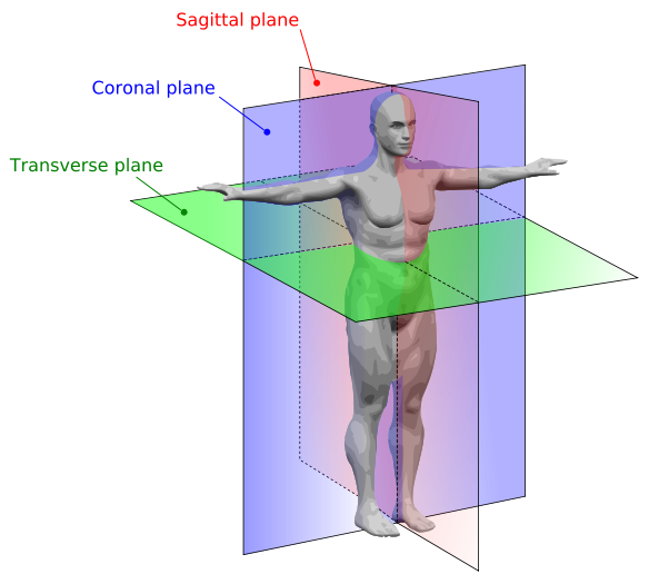
လူတွေရဲ့ လက်မှာ လှုပ်ရှားနိုင်တဲ့ ပုံစံ (degrees of freedom) ဘယ်နှစ်မျိုး ရှိလဲလို့ စဉ်းစား ဘူးပါသလား။ Saeed Benjamin Niku ရေးတဲ့ စာအုပ် တစ်အုပ် ဖြစ်တဲ့ Introduction to Robotics -Analysis, Control, Applications ထဲမှာ ဖတ်မိတဲ့ ဟာ တစ်ချို့ကို ပြန်ပြီး ထုတ်နုတ် တင်ပြ ချင်ပါတယ်။ လူ့ လက်မှာ ပခုံး၊ တံတောင်ဆစ် နဲ့ လက်ကောက်ဝတ် တွေက ကိုယ်၊ လက်မောင်း၊ လက်ဖျံ၊ လက်ဖဝါး တွေကို ဆက်ထား ပေးတဲ့ အဆက် နေရာတွေပါ။ ပခုံး က သုံးမျိုး လှုပ်နိုင်ပါတယ်။ coronal plane အတိုင်း အပေါ်အောက် လှုပ်လို့ရ သလို၊ transverse plane အတိုင်း ရှေ့နောက် လွှဲလို့ လဲရနိုင်ပြီး၊ လက်မောင်း ဝင်ရိုးမှာ လှည့်လို့ လည်း ရပါတယ်။ လူတွေရဲ့ ခန္ဓာဗေဒ ပြင်ညီ အခေါ်အဝေါ် ကို အောက်က Wikipedia က ပုံမှာ တွေ့နိုင်ပါတယ်။
တံတောင်ဆစ် ကတော့ အကွေး၊ အဆန့် တစ်မျိုးပဲ လှုပ်လို့ရတာပါ။ လက်ကောက်ဝတ် ကလဲ သုံးမျိုး လှုပ်နိုင်ပါတယ်။ အပေါ်အောက် လှုပ်တာ၊ ဘေးတိုက် လှုပ်တာ နဲ့ လက်ဖျံ တလျှောက် လှည့်တာ တွေ ဖြစ်ပါတယ်။ ဒါ့ကြောင့် လက်ချောင်းတွေကို ထည့်မစဉ်းစားဘူးဆိုရင် လူတွေရဲ့ လက်မှာ လှုပ်ရှားနိုင်တဲ့ ပုံစံ (degrees of freedom) ခုနှစ်မျိုး ရှိတယ်လို့ ပြောနိုင်ပါတယ်။